Measuring Kick — Current Capture, Accelerometers and a Repeatable Bench Rig

Volumes 2 to 5 rest on a lumped model and on makers’ data for parts other than the ones in the gun. This volume replaces those numbers with measurements. It is written for the instruments in the project’s lab: a Digilent Analog Discovery Pro ADP3450 (four analogue channels) and an Analog Discovery 2 as the oscilloscopes and logic analysers, several programmable bench supplies (one controlled over Bluetooth, the others over USB), a 50 A linear supply, and the usual meters.¹ Every measurement here can be made with them plus a shunt resistor, an accelerometer breakout and some string.

6.1 What to measure, and why

Table 1 — What to measure, and why

Quantity	Instrument	What it tells you
Coil current against time	Shunt into a scope channel	Arrival time (the cusp), current at landing, steady current and hence hot resistance, release time
Drain voltage against time	Scope channel through a ×10 probe	Clamp voltage, decay time, whether the switch is within its rating
Energy per shot	Math channel: supply voltage × current, integrated	Heat budget (Volume 4)
Acceleration of the gun or test mass	Analogue accelerometer into a scope channel	Peak and duration of the kick, impulse of the impact phase
Striker position or speed	High-speed video, optical or Hall sensor	Impact speed, return time
Sound	Microphone into a scope channel, or a sound-level meter	Effect of dampers and stops

Current and acceleration on one timebase, triggered by the firmware’s own pin, are the core. Everything else refines them.

6.2 Why a ballistic pendulum will not do

The textbook way to measure an impulse is to hang the object as a pendulum and measure its swing. For a solenoid kick that measures almost nothing. Momentum is conserved inside the gun: the coil pushes the gun forward while it accelerates the striker, and the stop pushes it back by the same amount when the striker lands (Volume 5). When the striker comes to rest against the stop, the gun is at rest too. A pendulum with a period of a second or two integrates over the whole shot and sees the sum, which is zero apart from small second-order effects.

What can be measured is the impact phase on its own: the momentum the striker gives up at the stop, and how fast. That needs a sensor with a bandwidth well above the impact’s inverse duration, which is an accelerometer, and an integration window that brackets the impact. A hanging test mass is still the right fixture, because it decouples the measurement from the bench and makes the integration meaningful; it is just not read by its swing.

6.3 Coil current

Shunt. A low-side shunt between the MOSFET source and ground is the simplest current sensor. At 3 A, a 0.1 Ω shunt gives 0.3 V, a comfortable signal, and dissipates 0.9 W during the pulse, a few hundred milliwatts on average at most firing rates; a 10 mΩ shunt gives 30 mV and is better when the shunt’s own drop matters. Use a four-terminal or a low-inductance metal-strip resistor and take the voltage from its pads, not from the ground plane.

The Analog Discovery Pro ADP3450. Digilent’s specification gives it four single-ended analogue inputs on BNC, 14-bit conversion, a bandwidth of at least 55 MHz, up to 125 MS/s per channel, and a buffer of up to 32 MS per channel in its standard mode. Its inputs have two ranges: 2 V peak-to-peak with ±1 V of offset at 200 mV/div and below, and ±25 V with respect to ground above that, with overvoltage protection to ±50 V DC.² A solenoid shot lasts tens of milliseconds and its interesting edges take tens of microseconds, so a sample rate of 1 to 10 MS/s is ample, and at those rates the buffer holds seconds of data: a whole burst of automatic fire in one capture. In its stand-alone Linux mode the buffer is limited to 32,768 samples, so long captures are made from WaveForms on a computer. It also has 16 digital I/O, usable as a logic analyser on the firmware’s sync and trigger pins, and two waveform generators.²

It has no current input. Coil current is captured as a voltage across a shunt, and because the inputs are single-ended the shunt belongs on the low side, between the MOSFET source and ground, where its voltage is referenced to the scope’s ground. A high-side shunt would need two channels and a math difference, and with the shunt sitting at 24 V of common mode the ±25 V range resolves only about 3 mV per step: a 10 mΩ shunt carrying 3 A gives 30 mV, ten steps. Where the circuit cannot be broken, a clamp-on DC current probe with a BNC output goes into a channel instead.

Triggering. Have the firmware raise a spare pin at the moment it energises the solenoid, and trigger the scope on that pin with a few milliseconds of pre-trigger. Triggering on the current itself works too, but a firmware sync makes the trigger-to-landing latency visible.

6.4 Drain voltage and the clamp

The MOSFET’s drain swings from near zero when on to the supply voltage plus the clamp voltage at turn-off: about 25 V with a plain diode on a 24 V supply, about 49 V with a 24 V Zener in series (Volume 4). The second exceeds the Analog Discovery’s ±25 V input range and approaches its ±50 V protection. Measure the drain through a ×10 probe, or not at all. The decay of the drain voltage back to the supply marks the end of the coil current, which is the clamp’s whole job; comparing it with and without the Zener measures what the clamp buys.

6.5 What one shot’s traces tell you

A current trace for one shot should look like the model’s (Volume 4): a rise on the open-plunger time constant, a dip while the plunger moves, a cusp at landing, a climb to V/R, and a decay after turn-off. Read from it:

1. Start delay, trigger to the first departure from the pure L/R rise: how long the coil takes to beat the spring.
2. Arrival time, trigger to the cusp. The basis of the pulse width.
3. Current at landing, the bottom of the cusp. A deep cusp means a fast plunger.
4. Steady current, I_ss = V/R_hot. Track it through a burst to watch the coil heat: R_hot = V/I_ss, and ΔT = (R_hot/R_cold − 1)/0.00393 (Volume 3).
5. Release time, turn-off to zero current.
6. Energy per shot, the integral of supply voltage times current over the shot, which the scope’s math channel can compute.

Ten shots at each setting give the spread, and the spread of arrival time is the best single measure of how consistently a part starts.

6.6 Acceleration: choosing the sensor

The impact is short. Volume 5 estimated contact times from about 0.1 ms for steel on steel to over a millisecond with a rubber pad. To see the shape of an impulse that short, the sensor needs a bandwidth of several kilohertz at least, and the sampling must be faster still.

• ADXL1002 or ADXL1001 (Analog Devices). Single-axis MEMS accelerometers with an analogue output, ±50 g and ±100 g respectively, a “linear frequency response range from dc to 11 kHz (3 dB point)” and a resonant frequency of 21 kHz, with a noise density of 25 µg/√Hz for the ADXL1002.³ An analogue output can go straight into a scope channel alongside the coil current, on the same timebase, sampled as fast as wanted. Analog Devices sells an evaluation board, EVAL-ADXL1002Z.³ This is the right class of sensor for this job.
• ADXL375 (Analog Devices). A three-axis digital accelerometer, ±200 g, with a bandwidth “of up to 1 kHz” and output data rates up to 3200 Hz over SPI or I²C.⁴ Adafruit sells it on a breakout, product 5374, for $24.95 as of 2026-10-18.⁵ Its range will not clip at a striker’s stop, but at 3200 samples a second it takes one reading every 0.3 ms and cannot resolve a 0.1 ms impact’s shape; it will under-read the peak. It is useful for logging the gun’s motion over a burst, not for the impact itself.
• General-purpose IMUs of the ±16 g class clip on a hard impact near the stop and sample too slowly. They are fine for aiming, not for this.

A rough magnitude check for the hanging-mass rig: a 20 g striker arriving at 2.4 m/s carries about 0.047 kg·m/s. On a 1.5 kg test mass that is a velocity change of about 31 mm/s. Delivered as a half-sine over 1 ms, the peak acceleration is about π·Δv/(2t), roughly 50 m/s² or 5 g; over 0.1 ms, roughly 50 g. Structural ringing at the sensor adds to that. A ±50 g sensor on the test mass, away from the stop, is about right; next to a steel-on-steel stop, ±100 g is safer.

6.7 Acceleration: mounting and reading it

• Mount it stiffly and lightly. A small breakout bonded with cyanoacrylate or screwed to a flat, rigid spot. Foam tape or a loose board acts as a filter and adds resonances of its own.
• Align the sensing axis with the striker’s axis, and record the sign convention: positive toward the shooter.
• Choose the location for the question. On the test mass’s centre, the trace is the rigid-body motion, which is what the integration needs. On a printed shell’s panel, it is the panel’s vibration, which is what the noise is. On the stock or the grip, it is close to what the shooter feels.
• Integrate only across the impact. Remove the pre-trigger offset, then integrate acceleration from just before the impact to just after it. The area is the velocity change the impact gave the mass, and that times the mass is the impulse of the impact phase. Integrating across the whole shot returns to zero, as Section 6.2 explains, apart from drift.
• Compare like with like. Peak acceleration depends on contact stiffness and on where the sensor is; the integrated impulse depends on neither. Report both.

6.8 Striker speed and position

The current cusp already gives the arrival time. For the speed:

• High-speed video. A phone’s slow-motion mode records at a few hundred frames a second, enough for two or three frames across a 10 ms stroke at 240 frames a second. A scale behind the striker and a short exposure under bright light make the frames readable. A dedicated high-speed camera does much better; none is listed in the lab.
• A slotted optical switch or a Hall sensor a known distance before the stop gives a timing edge on a logic channel; two of them give a speed.
• From the model. Once a part’s measured arrival time and moving mass are known, the lumped model’s coil parameters can be adjusted until it reproduces the measurement, and then its impact speed is a reasonable estimate.

6.9 Sound

A microphone into a spare scope channel, or a sound-level meter at a fixed distance, records the effect of each damper and stop. The comparison that matters is between configurations measured the same way on the same day; absolute sound-pressure levels are not needed for that.

6.10 The rig

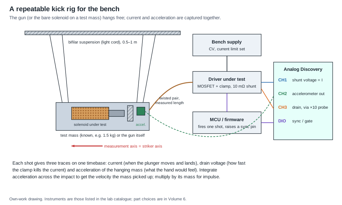
• Suspension. Two pairs of light cords, 0.5 to 1 m long, from a rigid beam, so the mass hangs level and swings only along the striker axis. The suspension’s own period is a second or more, far longer than a shot, so during the impact the mass is effectively free.
• Test mass. A block of aluminium or steel of about 1 to 2 kg, roughly the weight of the finished gun, with the solenoid and its stops bolted to it in the arrangement the gun will use. Once a gun exists, hang the gun itself.
• Supply and driver. The bench supply in constant-voltage mode with its current limit set just above the expected peak, which also protects the coil if the driver sticks on. The driver is the one under development, so that the rig measures the gun’s real electronics.
• Wiring. A twisted pair of known length from driver to coil, the same length as in the gun, because wiring resistance is one of the variables (Volume 3).
• Logging. WaveForms’ script editor can repeat a capture and save each shot’s traces to a file; a short script that fires, captures and saves ten shots per setting makes the comparisons honest.

6.11 A test plan

A first session on a new solenoid and striker, in order:

1. Characterise the solenoid itself (Volume 3, steps 1 to 4).
2. Mount it on the test mass with its striker and stops; record the moving mass.
3. At the working supply voltage, fire ten single shots with a long pulse (50 ms). Read the arrival time and its spread.
4. Set the pulse to arrival plus 3 ms. Fire ten more. Confirm that the integrated impulse is the same as with the long pulse and that the energy per shot has fallen.
5. Repeat step 4 with the Zener clamp fitted. Read the release time and check the drain voltage against the MOSFET’s rating.
6. Fire a burst at the firmware’s automatic rate for 30 seconds, logging the steady current of each shot. Plot the inferred winding temperature against the frame sensor’s reading.
7. Change one mechanical variable at a time (striker mass, rear-stop damper, forward-stop damper, spring) and repeat step 4 and the sound measurement.
8. Write every result into the record sheet (Volume 3), and the chosen pulse width and current into the gun’s firmware profile.

The USB-controlled supplies can be stepped from the same script that fires and captures, so a voltage sweep runs unattended; the Bluetooth-controlled supply is best kept for the logic and sensor rail, which should not move during a sweep. Volume 8 uses this plan to rank the candidate solenoids against each other.

6.12 Why this, and why not the others

Table 2 — Why this, and why not the others

Choice	Picked	Alternatives and why they lost
Current sensing	Low-side metal-strip shunt, 0.1 Ω (or 10 mΩ when its drop matters), into one ADP3450 channel	High-side shunt across two channels: poor resolution at 24 V common mode on single-ended ±25 V inputs. Hall-effect current-sensor IC on the board: adds its own bandwidth limit and offset, and is a design choice for the driver, not a lab instrument. Clamp-on probe: good where the circuit cannot be opened, but not on the lab list; buy only if needed
Acceleration sensor	ADXL1002 (±50 g) or ADXL1001 (±100 g) analogue, on the scope	ADXL375: will not clip, but 3200 samples a second cannot resolve a 0.1–1 ms impact. ±16 g IMUs: clip and sample too slowly. Piezoelectric accelerometer: excellent bandwidth, but needs a charge or IEPE amplifier the lab does not list
Impulse method	Integrate acceleration across the impact on a hanging test mass	Ballistic pendulum: reads almost nothing (Section 6.2). Load cell under the stop: measures force at the stop well but adds compliance that changes the hit
Supply during tests	Programmable bench supply in constant-voltage mode, current limit just above the peak	The supply’s constant-current mode: its loop is far slower than a 10 ms pulse. The 50 A linear supply: kept for low-impedance pulse tests where droop must be ruled out

6.13 What could not be verified

• The price and availability of EVAL-ADXL1002Z were not captured.
• Impact durations remain estimates until the rig measures them.

Sources

Footnotes

1. Project lab catalogue, _shared/lab_capability.md, Electronics section, as of 2026-10-18; bench-gear decision of 18 October 2026 (ADP3450; programmable supplies, one Bluetooth-controlled and the rest USB-controlled; models not recorded). ↩

2. Digilent, Analog Discovery Pro (ADP3450/ADP3250) Specifications, revision 0924, copy at https://assets.testequity.com/te1/Documents/pdf/Digilent_Analog-Discovery-Pro-ADP3450-ADP3250_Specifications_0924.pdf, read 2026-10-18 (Digilent’s own reference page at https://digilent.com/reference/test-and-measurement/analog-discovery-pro-3x50/specifications refused automated access). ↩ ↩²

3. Analog Devices, ADXL1001/ADXL1002 data sheet, https://www.analog.com/media/en/technical-documentation/data-sheets/adxl1001-1002.pdf, read 2026-10-18 (features, ordering guide, evaluation boards). ↩ ↩²

4. Analog Devices, ADXL375 data sheet, https://www.analog.com/media/en/technical-documentation/data-sheets/ADXL375.PDF, read 2026-10-18. ↩

5. Adafruit, “ADXL375 - High G Accelerometer (+-200g) with I2C and SPI - STEMMA QT / Qwiic”, product 5374, https://www.adafruit.com/product/5374, read 2026-10-18. ↩